Dec 14th, 2025: [EN] Build a map to compare metrics by country or region with ES|QL

[Nathan_Reese]

Kibana map tutorial "Build a map to compare metrics by country or region" creates a map using Elasticsearch’s DSL querying. Recent ES|QL functions LOOKUP JOIN (8.18) and ST_GEOTILE (9.2) allow the map in this tutorial to be re-created with ES|QL.

Below are the steps to re-create the tutorial map with ES|QL. Then, the steps go beyond what is possible in the original tutorial and normalizes the choropleth layer by country population.

Prerequisites

• If you don’t already have Kibana, set it up with our free trial.
• This tutorial requires the web logs sample data set.
• You must have the correct privileges for creating a map and creating an index.

Step 1. Create a map

• Go to Dashboards.
• Click Create dashboard.
• Set the time range to Last 7 days.
• Click the Add button and select New panel. Finally click Maps

Step 2. Add a choropleth layer

The first layer you’ll add is a choropleth layer to shade world countries by web log traffic. Darker shades will symbolize countries with more web log traffic, and lighter shades will symbolize countries with less traffic.

Index world countries

1. Download world countries GeoJSON file
2. In Kibana maps, click Add layer
3. Select Upload file
4. Select world countries GeoJSON file in file selector
5. Set Index name to world_countries
6. Open Advanced section
7. Set Index settings to { "index.mode": "lookup" }.
   
   
   
8. Click Import file
9. When the file import finishes, click cancel

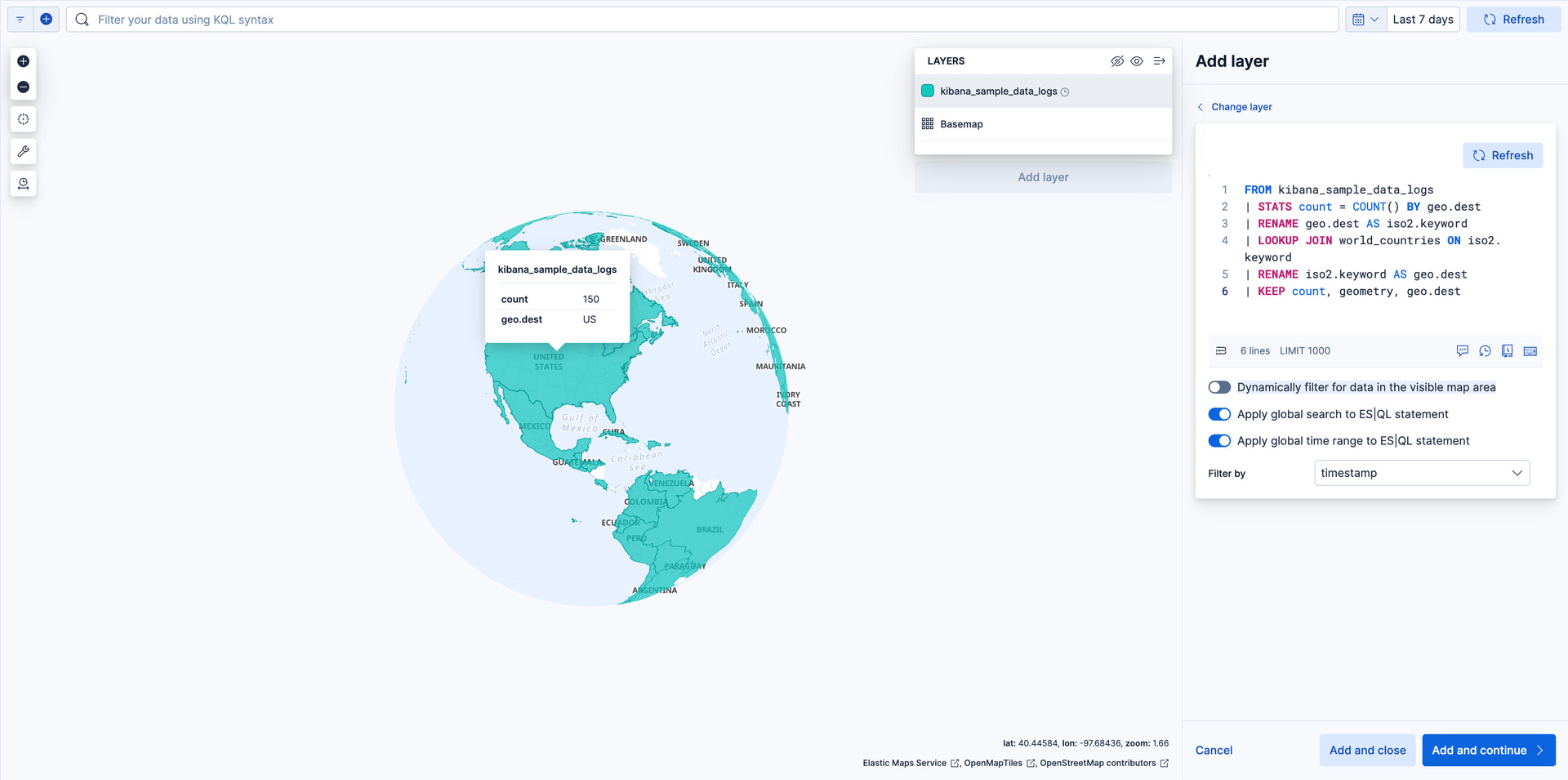
Add the choropleth layer

1. Click Add layer
2. Select ES|QL
3. Set ES|QL statement to

FROM kibana_sample_data_logs 
| STATS count = COUNT() BY geo.dest 
| RENAME geo.dest AS iso2.keyword 
| LOOKUP JOIN world_countries ON iso2.keyword 
| RENAME iso2.keyword AS geo.dest 
| KEEP count, geometry, geo.dest

4. Click Run query in ES|QL editor
5. Unselect Dynamically filter for data in the visible map area
   
   
   
6. Click Add and continue
7. In Layer settings, set:
   1. Name to Total Requests by Destination.
   2. Opacity to 50%.
8. In Layer style
   1. Set Fill color to By value by count. Select "grey to black" color gradient.
   2. Set Border color to "white". 4.
9. Click Keep changes. Your map should now look like
   
   
   

Step 3. Add layers for the Elasticsearch data

To avoid overwhelming the user with too much data at once, you'll add two layers for the Elasticsearch data. The first layer will display individual documents when users zoom in on the map. The second layer will display aggregated data when users zoom the map out.

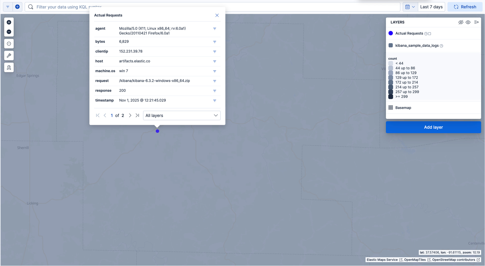
Add a layer for individual documents

This layer displays web log documents as points.
The layer is only visible when users zoom in.

1. Click Add layer
2. Select ES|QL
3. Set ES|QL statement to

FROM kibana_sample_data_logs 
| KEEP geo.coordinates, agent, bytes, clientip, 
       host, machine.os, request, response, timestamp 
| LIMIT 10000

4. Click Run query in ES|QL editor
5. Click Add and continue
6. In Layer settings, set:
   1. Name to Actual Requests.
   2. Visibility to the range [9, 24].
7. In Layer style, set:
   1. Fill color to #2200FF .
   2. Border width to 0.
8. Click Keep changes. Your map should now look like
   
   
   

Add a layer for aggregated data

You'll create a layer for aggregated data and make it visible only when the map is zoomed out. Darker colors will symbolize grids with more web log traffic, and lighter colors will symbolize grids with less traffic. Larger circles will symbolize grids with more total bytes transferred, and smaller circles will symbolize grids with less bytes transferred.

1. Click Add layer
2. Select ES|QL
3. Set ES|QL statement to

FROM kibana_sample_data_logs  
| EVAL geotile = ST_GEOTILE(geo.coordinates, 6) 
| STATS count = COUNT(geotile), 
        sumOfBytes = SUM(bytes), 
        centroid = ST_CENTROID_AGG(geo.coordinates) BY geotile

4. Click Run query in ES|QL editor
5. Click Add and continue
6. In Layer settings, set:
   1. Name to Total Requests and Bytes.
   2. Visibility to the range [0, 9].
7. In Layer style, set:
   1. Fill color to By value by count
   2. Border width to 0.
   3. Symbol size to By value by sumOfBytes. Set the min size to 7 and the max size to 25.
   4. Label to By value by count
8. Click Keep changes. Your map should now look like
   
   
   

Step 4. Normalize choropleth layer by country population

The choropleth layer created in step 2 shades world countries by web log traffic. Comparing counts between countries is not a fair comparison since countries have varying populations. Large populations likely have more web traffic then small populations. Instead, you want to shade world countries by web log traffic adjusted for population.

ES|QL makes it possible to normalize web log counts by taking into account the total population of each country. Instead of visualizing web log counts, we will visualize web log counts per 100,000 people. Now, we can compare normalized counts between countries.

Index world country populations

1. Download populations_2024.csv file. This file is derived from World Bank Group.
2. In Kibana, go to File upload using the global search field.
3. Select populations_2024.csv in file selector
4. Set New index name to populations
5. Click Import

Add population field to world_countries index

Use enrich processor to add populations to the world countries set.

1. Go to Developer tools using the navigation menu or global search field.

2. Create a match enrichment policy

   PUT /_enrich/policy/population_lookup
   {
     "match": {
       "indices": "populations",
       "match_field": "iso3",
       "enrich_fields": [ "population_2024"]
     }
   }
   

3. To initialize the policy, run:

   POST /_enrich/policy/population_lookup/_execute
   

4. To create a ingest pipeline, run:

   PUT _ingest/pipeline/add_population_to_world_countries
   {
     "processors": [
       {
         "enrich": {
           "field": "iso3",
           "policy_name": "population_lookup",
           "target_field": "population",
           "ignore_missing": true,
           "ignore_failure": true
         }
       }
     ]
   }
   

5. To add population data to world countries, run:

   POST world_countries/_update_by_query?pipeline=add_population_to_world_countries
   

6. View world_countries index in Discover. Each row now includes population.population_2024 column
   
   

   

Normalize count per population in ES|QL statement

1. Click edit button for Total Requests by Destination layer.
2. Replace ES|QL statement with

FROM kibana_sample_data_logs 
| STATS count = COUNT() BY geo.dest 
| RENAME geo.dest AS iso2.keyword 
| LOOKUP JOIN world_countries ON iso2.keyword 
| RENAME iso2.keyword AS geo.dest 
| KEEP count, geometry, geo.dest, population.population_2024 
| EVAL normalized_count = TO_DOUBLE(count) / population.population_2024 * 100000

3. Click Run query in ES|QL editor
4. In Layer style set Fill color to By value by normalized_count.
5. Click Keep changes.

Your map should now look like

Note: You may have guessed why not importing the populations CSV with the lookup setting to perform a second LOOKUP JOIN to the map query. That would work! but mind that there is a performance penalty on each additional join.