ML calculates wrong averages on pre-aggregated data

[guysmoilov]

Hi everyone, I would like some help or an explanation regarding how to work using pre-aggregated data for ML.

Scenario: We’re indexing pre-aggregated data to Elasticsearch. Each document has the following (relevant) fields:
• PageLoadEventCount: how many page load events were aggregated into this document.
• TotalResponseTime: The milliseconds spent waiting for a response during the page load, summed over all events aggregated into this document. To get a proper average response time per page load, this number should be divided by PageLoadEventCount
• Browser
• Timestamp
• Other interesting influencer fields, e.g. Country

I defined an ML job intended to monitor the average response time of page loads. Note that I included the summary_count_field_name, which according to Elasticsearch’s documentation is intended exactly for the use case of analyzing pre-aggregated data. The ML job configuration can be seen here:

{
"job_id" : "ml-avg-response-time-2",
"job_type" : "anomaly_detector",
"job_version" : "5.5.2",
"description" : "",
"create_time" : 1505666647208,
"finished_time" : 1505668033228,
"analysis_config" : {
"bucket_span" : "5m",
"summary_count_field_name" : "PageLoadEventCount",
"detectors" : [{
"detector_description" : "high_mean(TotalResponseTime) over Browser",
"function" : "high_mean",
"field_name" : "TotalResponseTime",
"over_field_name" : "Browser",
"detector_rules" : ,
"detector_index" : 0
}
],
"influencers" : [
"BrowserGroup",
"Country",
"Browser",
"OperatingSystem"
]
},
"data_description" : {
"time_field" : "Timestamp",
"time_format" : "epoch_ms"
},
"model_plot_config" : {
"enabled" : true
},
"model_snapshot_retention_days" : 1,
"model_snapshot_id" : "1507031088",
"results_index_name" : "shared",
"data_counts" : {
"job_id" : "ml-avg-response-time-2",
"processed_record_count" : 146247799,
"processed_field_count" : 10641937,
"input_bytes" : 4349257045,
"input_field_count" : 10641937,
"invalid_date_count" : 0,
"missing_field_count" : 866844857,
"out_of_order_timestamp_count" : 0,
"empty_bucket_count" : 0,
"sparse_bucket_count" : 258,
"bucket_count" : 161864,
"earliest_record_timestamp" : 1504181025000,
"latest_record_timestamp" : 1507030349000,
"last_data_time" : 1507030950314,
"latest_empty_bucket_timestamp" : 1506705300000,
"latest_sparse_bucket_timestamp" : 1505725200000,
"input_record_count" : 146247799
},
"model_size_stats" : {
"job_id" : "ml-avg-response-time-2",
"result_type" : "model_size_stats",
"model_bytes" : 1089490,
"total_by_field_count" : 3,
"total_over_field_count" : 133,
"total_partition_field_count" : 2,
"bucket_allocation_failures_count" : 0,
"memory_status" : "ok",
"log_time" : 1507031088000,
"timestamp" : 1507029900000
},
"datafeed_config" : {
"datafeed_id" : "datafeed-ml-avg-response-time-2",
"job_id" : "ml-avg-response-time-2",
"query_delay" : "600s",
"frequency" : "150s",
"indices" : [
"singledim_agguser*"
],
"types" : [
"singledim_agguser"
],
"query" : {
"match_all" : {
"boost" : 1
}
},
"scroll_size" : 1000,
"chunking_config" : {
"mode" : "auto"
},
"state" : "stopped"
},
"state" : "closed"
}

Looking at the anomaly explorer, this is what I saw:

It claims a spike of avg. response time of about 40 seconds! Looking at the raw data however, I see that this is simply caused by the average not being properly calculated according to the number of page load events:

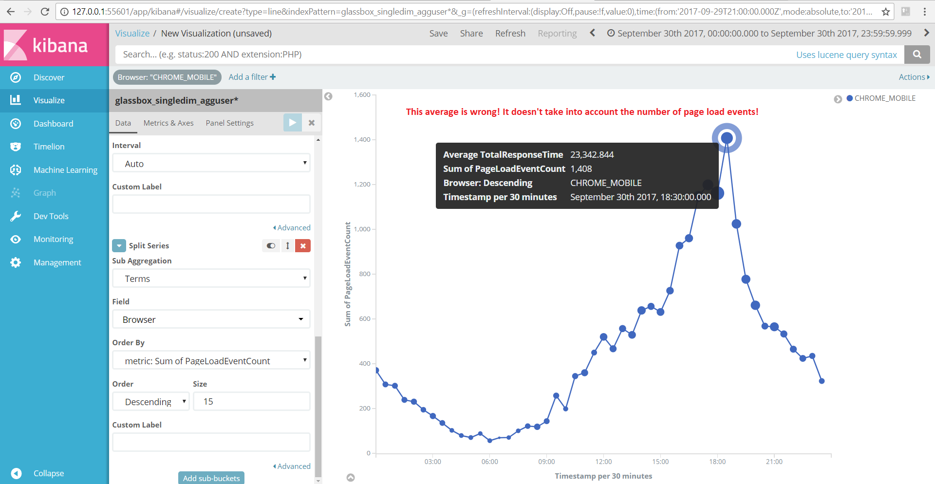
Am I missing something here? Shouldn't the high_mean detector take the summary_count_field_name into account when calculating an average?
Also, will the anomaly's probability be weighted according to how many events took part in the data which generated the anomaly? If not, the anomalies will be very susceptible to outliers when traffic is low.

Thanks

[dmitri (Dimitris Athanasiou)]

Hi,

The support for pre-aggregated data expects that the pre-aggregated value was calculated using the same aggregation function as that of the ML detector. If that was not the case, it would not be possible to provide pre-aggregated averages, for example.

In your example, it should be that the value of TotalResponseTime is already the average instead of the sum of the response times. You can use sum functions without an issue. But, if what you want is to detect anomalies with regard to the mean, you will have to provide the mean values yourself.

One way to achieve that would be to make use of script_fields in the datafeed config. You can find more information about this here.

[guysmoilov]

Thanks for the reply.

We initially did do what you suggest, and relied on scripts to calculate the average during queries, but in practice the performance penalty was staggering compared to just saving sums and doing the division in the client side post-query. Is there no intention to support the kind of behaviour I'm looking for? Otherwise, we will be forced to add another field only for the detector, since as I said query time suffered enormously when we used scripts, so we won't change the existing field's behaviour.

Anyway, I'll try to use the script_fields as you suggested, and hope that the query performance doesn't suffer too much.

Also, is the anomaly probability and severity weighted according to the event count field?

[dmitri (Dimitris Athanasiou)]

ML is designed to work with either the user's raw data or with output from using elasticsearch's APIs (e.g. scripts, aggs, etc.). I am not aware of your use case, but I would recommend exploring and evaluating available options. On top of the ones you mentioned, I would add the option of replacing the total response time with the average during indexing (if total response time is not otherwise interesting to you).

Also, when it comes to using script_fields, if you intend to run the job in real-time mode, compare the cost of the query during the historical data analysis as opposed to the real-time mode. I would expect that to be lighter.

The event count is not used to weigh the anomaly probability or severity. In this instance it explains the number of observations that made up the total response time. This allows us to be more granular and accurate to our modelling. A measurement that represents a single observation will have a different impact than a measurement that represents multiple observations.

[guysmoilov]

Wait, I'm a bit confused regarding the anomaly severity calculation.
Please imagine the following list of documents (let's assume the respTime is indeed saved as an average):

• { respTime: 500, eventCount: 1000, timestamp: 1 }
• { respTime: 500, eventCount: 3000, timestamp: 2 }
• { respTime: 10000, eventCount: 3, timestamp: 3 }
• { respTime: 500, eventCount: 2000, timestamp: 4 }
• { respTime: 10000, eventCount: 1000, timestamp: 5 }

The third and fifth documents are technically both anomalous to the same degree if you look only at the average. However, I would like to see that the anomaly for the third event is low severity, since there are very few samples and it's likely an outlier, and that the anomaly in the fifth document is high severity. Without taking the number of samples into account, I have trouble seeing how we can ignore false positives.
So, my question now is - will this behave as I described?

[Tom_Veasey]

The way to think about our modelling of timestamped metrics is in terms of features which describe some user defined aggregate of the metric values which land in an interval of time. The time interval is the bucket span you select when you create the job. We typically don't care how these values are distributed between documents, although more on this later on. (One thing to note in this context is that we purposely only learn at a rate which is dependent on the time span and not the number of values you get per unit time. We found this is important because one often sees important variation between the values over significant time ranges even if their rate is high and we become confident too quickly if we learn at a fixed rate from each individual value.)

Thinking about how the modelling will behave on your example. The answer would depend on the bucket span you choose.

If you set the bucket span to be 1, in this example each document lands in its own bucket. The value of the feature for that bucket will depend on the aggregation you've chosen. If you chose sum then you'd get a feature value of 500 x 1000 in the first bucket, 500 x 3000 in the second bucket and so on. If you chose mean then the feature values would be 500, 500, 10000, etc. To your specific question, when we consider how unusual a mean value is we do consider the impact of the count in that statistic versus the typical count we've seen for historical values of that statistic. We do this by transforming the distribution we predict for that value. This is important because one usually expects the variance of the mean to decrease in proportion to the count of values it includes. We want to capture this effect so we don't say an unusual mean feature value only containing a relatively small number of metric values is necessarily anomalous.

Contrast this with if you choose a bucket span of 5. In this case, if you analyse the mean aggregate, we will compute the value for the feature as (500 x 6000 + 10000 x 1003) / 7003. In this case, the distribution of values between documents is not important since we only care about how unusual the feature.

It is also worth mentioning how an influencer will behave in this context. I wouldn't typically recommend using timestamp as an influencer, but for illustration purposes suppose you do. Note that this doesn't cause us to change how unusual we say the time interval is: this is always based on the feature value. However, we do ask ourselves the extent to which each distinct value of the timestamp, i.e. each document, has caused the mean value to be anomalous. The consideration is different for different aggregations, but in the case of mean it is strongly affected by count. So in this case if the mean value, i.e. (500 x 6000 + 10000 x 1003) / 7003, is unusually high we will recognise that this is due to the document with timestamp 5 and not with timestamp 3.

[guysmoilov]

Thanks for the detailed reply!

In the example I gave, I implicitly meant that each document lands in a distinct time bucket, according to the bucket span. Sorry that I didn't make that clear. I understand that the ML algorithm (justifiably) doesn't care how many documents are in each bucket, only the aggregation results for that whole bucket together. This is even doubly true in my case, since each document is an aggregation of several events anyway, and the actual doc count is completely meaningless.

So if I understood you correctly:

To your specific question, when we consider how unusual a mean value is we do consider the impact of the count in that statistic versus the typical count we've seen for historical values of that statistic. We do this by transforming the distribution we predict for that value. This is important because one usually expects the variance of the mean to decrease in proportion to the count of values it includes. We want to capture this effect so we don't say an unusual mean feature value only containing a relatively small number of metric values is necessarily anomalous.

This means that the answer to my question is basically "yes" - you take into account the law of large numbers / Markov inequality / Chernoff bound / whatever, as described by the doc count field, when deciding whether a bucket is anomalous.

[Tom_Veasey]

No problem, and exactly. We have to make some assumptions here, since we don't really have enough information to estimate correlations in the individual metric values, so essentially we are applying exactly this sort of effect. We also approximately capture this in the bounds we show if model plot is enabled, i.e. you should see the bounds grow/shrink for low/high (compared to typical) count buckets.